In a past life, I worked on an app that let users upload and share photos with friends and family. I’m amazed at how far technology has progressed since that time. It feels like magic that AI can “look” at a set of photos and “know” that they were taken at a child’s first birthday party or on a hike in the mountains. Natural language queries like “show me photos from my trip to the Statue of Liberty” or even “find that photo where I’m about to collide on the soccer field with another player” are no longer science fiction.
Our photo-sharing startup never reached millions of users, but I suspect that many of you reading this are working on systems that have. At that scale, it’s surprisingly easy to find yourself managing billions, or even tens of billions of user-generated items. If it’s a photo app, most users will have hundreds or thousands of photos. Power users or organizations might have tens or hundreds of thousands. If it’s not photos, it might be documents, notes, videos, or audio. The type of content varies, but the math is the same: millions of users, each contributing hundreds or thousands of items, and you’re quickly operating at billions-scale.
Even with just a few hundred items, users expect fast, accurate search. If they upload something, they want to find it immediately. If they search, they want results in the blink of an eye. Increasingly, basic keyword search isn’t enough. In the age of ChatGPT, users expect semantic search, with results based on the meaning of the content, not just filenames, metadata, keywords, or tags.
Some solutions to this problem assume that the entire dataset fits into memory on a single machine. Or, at most, they rely on a fast local SSD. Many of them don’t expect your data to be distributed across regions, or to be constantly changing, or to be part of a transactional system where consistency and freshness actually matter. They often come with significant limitations, like requiring writes to be batched, returning stale results, or needing specialized hardware to perform well.
CockroachDB was built with a different set of assumptions. As a distributed database, it expects data to live across multiple machines, which may span availability zones or even regions. It’s designed to scale linearly, so that adding more machines leads to proportionally higher throughput. And as a transactional SQL database, it prioritizes returning fresh data and supporting real-time updates. All of that has to be resilient to machine, disk, and network failures.
Read on to learn how we combined recent academic research with practical engineering to solve the semantic search problem at massive scale, with fresh, real-time results, by leveraging CockroachDB’s unique distributed architecture.
Embedding Meaning into Vectors
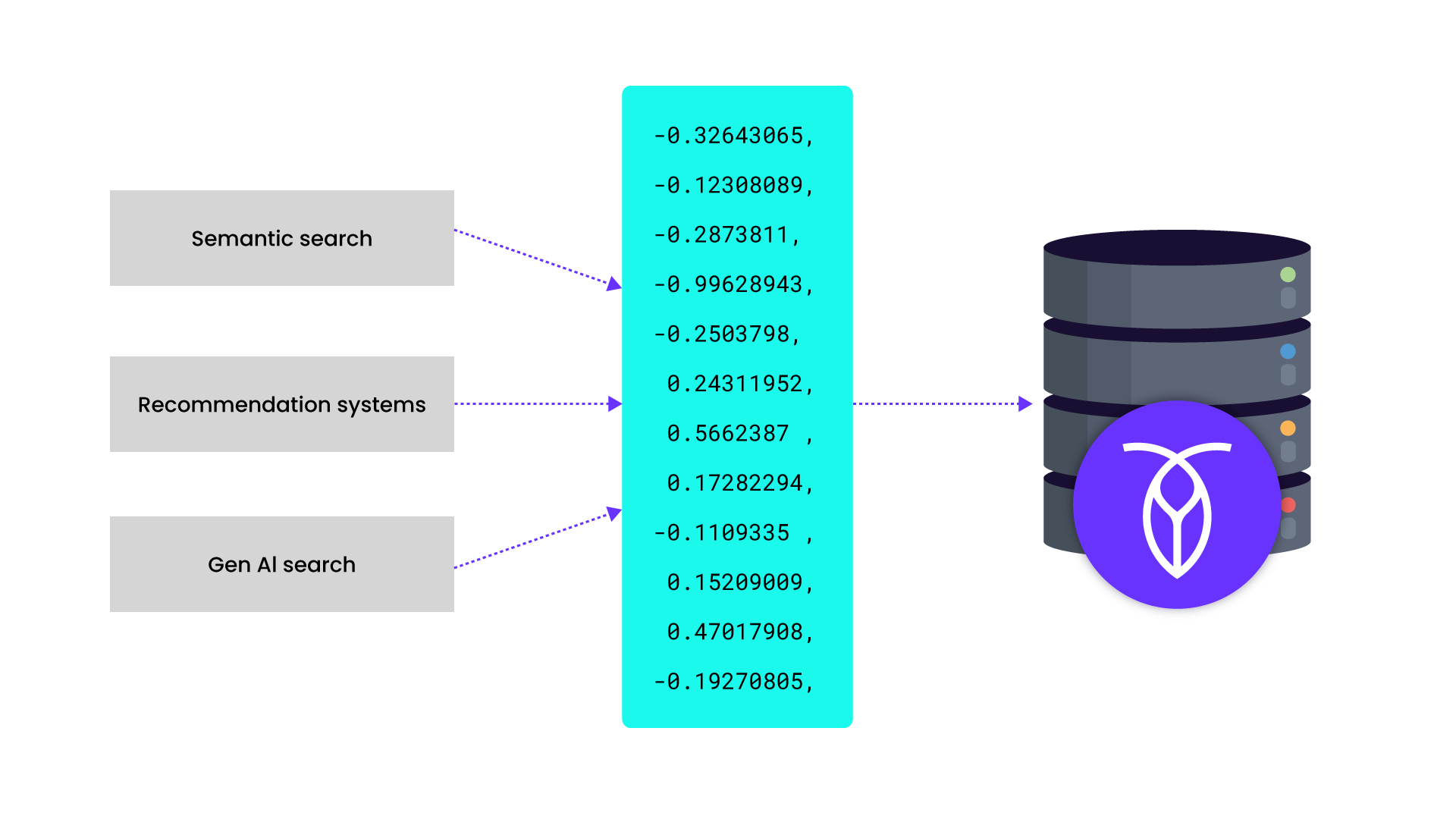
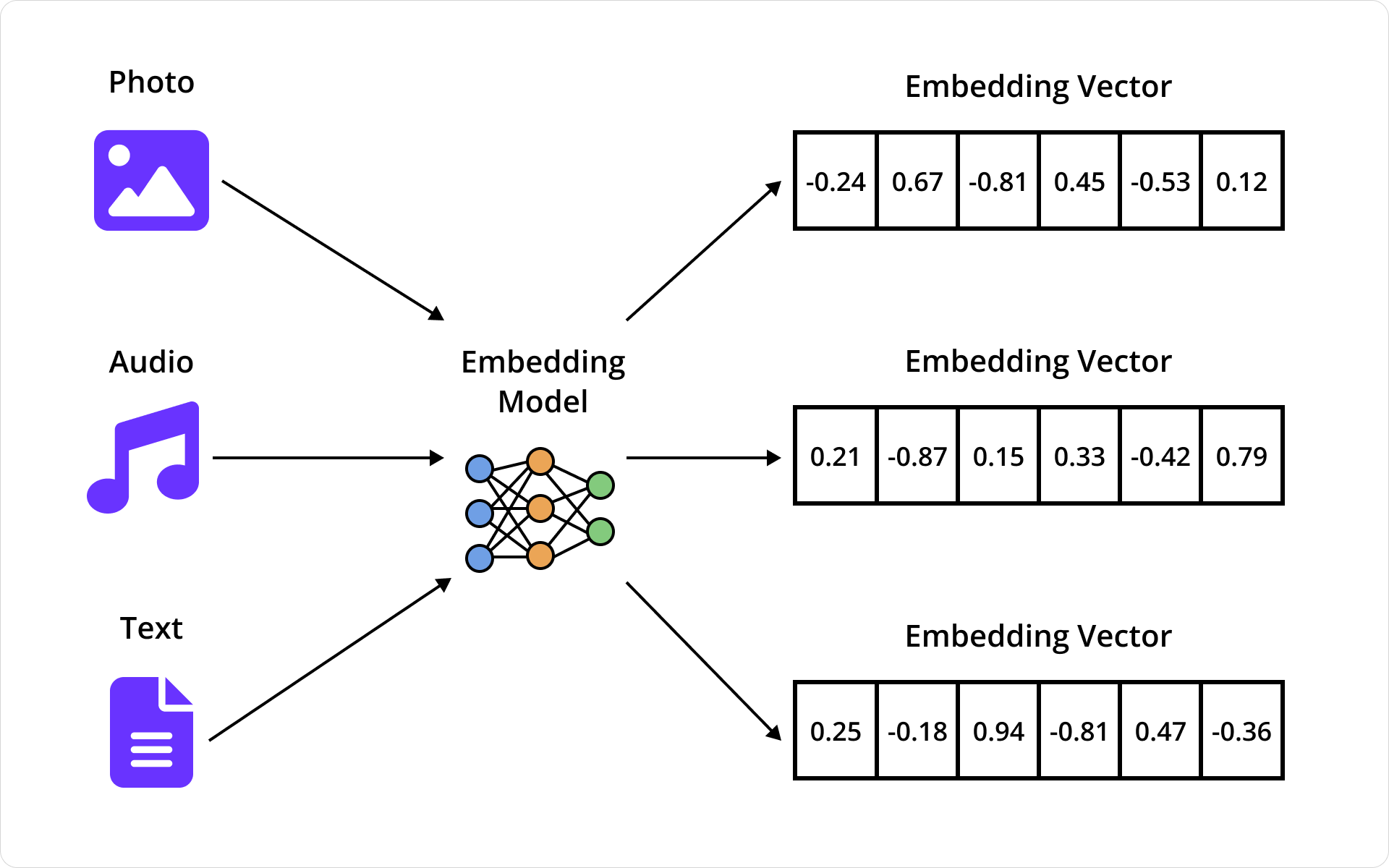
To start, it’s important to understand how systems can make sense of photos or search documents by meaning. Companies like OpenAI offer embedding models that convert an image, document, or other media into a long list of floating-point numbers – a vector – that captures its meaning. If two photos or documents are similar, say two beach photos, they’ll be mapped to vectors that are near each other in high-dimensional space.
Embedding meaning into vectors reduces complex problems like image recognition and semantic search into a simpler one: finding nearby vectors. These models are built on the same deep learning techniques that power systems like ChatGPT – large neural networks trained to capture meaning and context across many kinds of data.
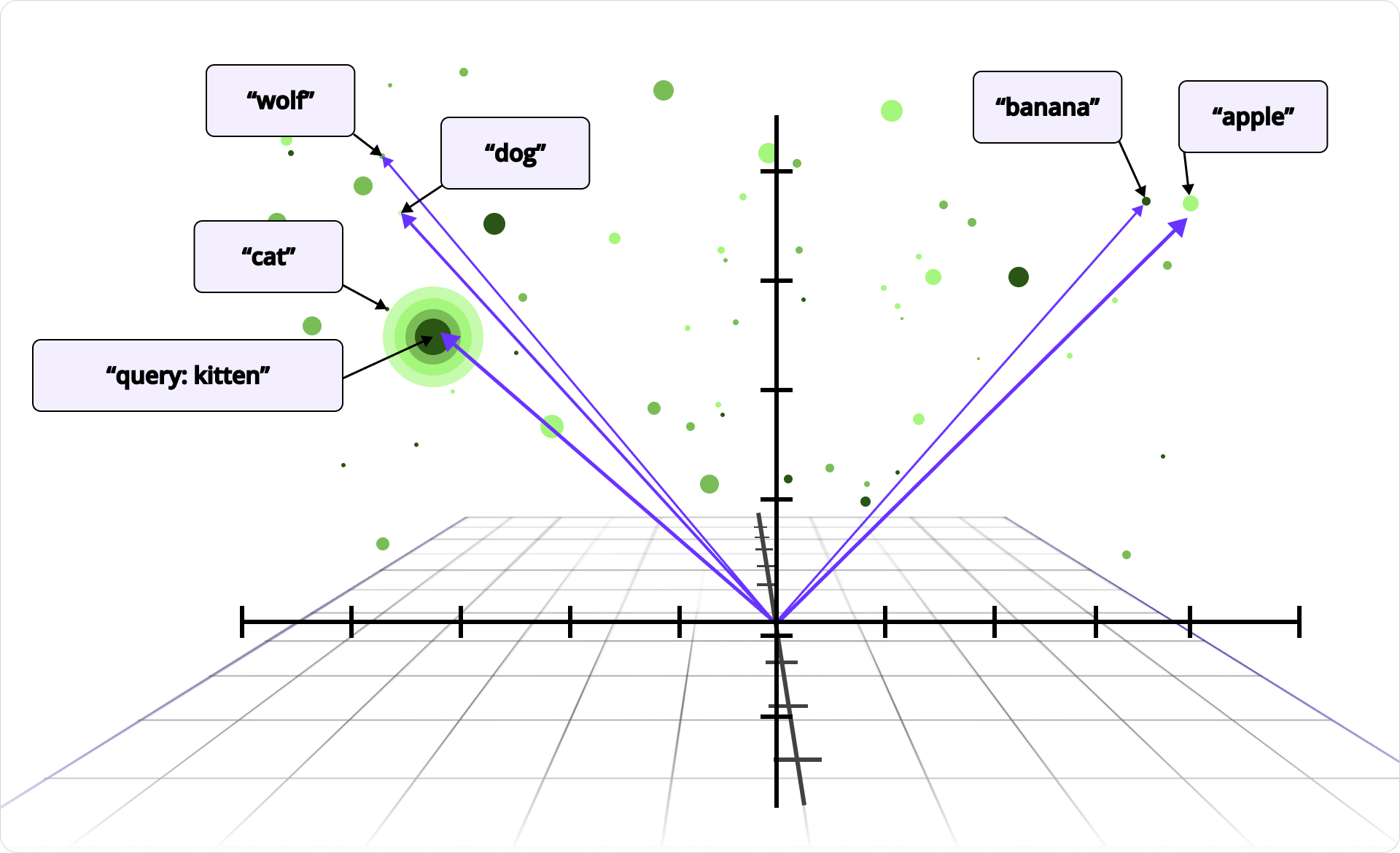
This even works across media types. Multimodal models embed text and images into the same vector space. So the word “beach” and an actual beach photo end up in the same region. When a user types “beach,” we can embed that query into a vector and search for nearby photo vectors. The closest matches are very likely to be related to the beach.
How Meaning is Indexed
Embedding vectors often have hundreds or thousands of dimensions that allow them to represent complex meaning. But that also makes them hard to search. Think about it: should beach photos come before or after food photos? What about photos of food at the beach? There’s no natural ordering for multi-dimensional vectors, the way there is for numbers or strings. That means traditional indexes don’t apply.
Instead of scanning for exact matches, semantic queries need to find vectors that are nearby in multi-dimensional space. At a small scale, brute-force search is often good enough – you can scan the dataset, compute distances, and return the closest matches. But as the number of vectors grows into the tens of thousands or beyond, that approach quickly becomes too slow to be practical.
Vector indexes address this by efficiently finding approximate nearest neighbors. These indexes trade a small amount of accuracy for a large gain in performance. While they don’t guarantee that the exact nearest vectors will be returned, the results are close enough to be useful, and the performance benefits make real-time search possible at scale.
Adapting Vector Indexing Algorithms for Distributed SQL
Even with a good vector indexing algorithm, plugging it into a distributed SQL database like CockroachDB isn’t straightforward. To support elastic scale, fault tolerance, and multi-region availability, any indexing algorithm needs to follow a set of architectural rules:
No central coordinator. Any node in the cluster should be able to serve reads and writes. The index can’t rely on a single leader to coordinate queries or updates.
No large in-memory structures. Index state must live in persistent storage. We can’t assume every node has gigabytes of RAM available for caching vectors, and we want to avoid long warm-up times spent building large in-memory structures. This is especially important for Serverless deployments.
Minimal network hops. Cross-node round-trips are expensive. Indexes that require sequential traversal across nodes can accumulate latency quickly and make performance unpredictable.
Sharding-compatible layout. Index data must map naturally to CockroachDB’s key-value ranges so it can be split, merged, and rebalanced like any other data.
No hot spots. As vector inserts and queries scale up, the index must avoid concentrating traffic on a single node or range. Load should be balanced across the cluster.
Incremental updates. The index must handle inserts and deletes in real time, without blocking queries, requiring large rebuilds, or hurting search quality.
These constraints ruled out many common approaches. We needed something that fit cleanly into CockroachDB’s execution model and harnessed the power of its distributed architecture. That’s where C-SPANN comes in.
Introducing C-SPANN
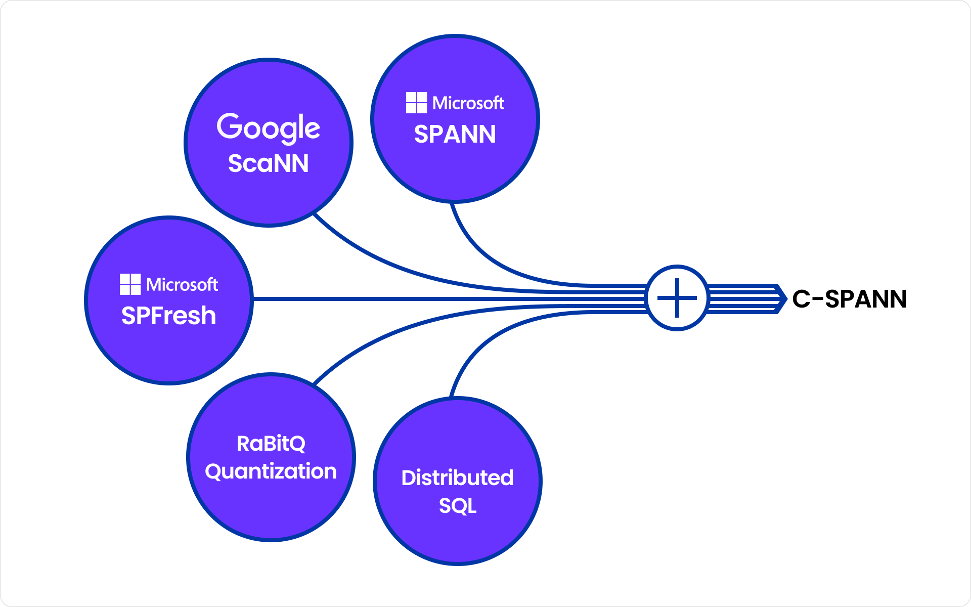
C-SPANN, short for CockroachDB SPANN, is a vector indexing algorithm that incorporates ideas from Microsoft’s SPANN and SPFresh papers, as well as Google’s ScaNN project.
At the core of C-SPANN is a hierarchical K-means tree. Vectors are grouped into partitions based on similarity, with each partition containing anywhere from dozens to hundreds of vectors. Each partition has a centroid, which is the average of the vectors it contains, representing their “center of mass”. Those centroids are recursively clustered into higher-level partitions, forming a tree that efficiently narrows the search space.
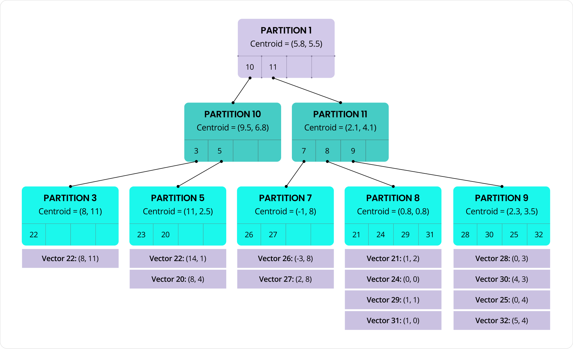
Each partition is stored as a self-contained unit in CockroachDB’s key-value layer, making the index naturally sharding-compatible. Partition data is laid out as a contiguous set of key-value rows within a CockroachDB range. As partitions are added, removed, or grow in size, the underlying ranges can be automatically split, merged, and rebalanced by the database, just like any other table data.
At query time, the search starts at the root of the tree. We compare the query vector to the centroids at that level, then descend into the partitions with the closest matches. This process repeats at each level until we reach the leaves, where we scan a small number of candidate vectors. Partitions at each level can be processed in parallel, helping to reduce latency. And because vectors within a partition are packed together and are similar by design, we can take advantage of SIMD CPU instructions to efficiently scan blocks of vectors.
Because the tree fanout is typically around 100, the structure remains wide and shallow. This keeps the number of levels (and therefore the number of network round-trips) small and predictable, even at large scale. An index with 1 million vectors requires just 3 levels; even one with 10 billion vectors needs only 5 levels. To reduce round-trips even further, the root partition can be cached in memory.
C-SPANN also avoids central coordination. Any node can serve queries or handle inserts and updates. The index structure lives in persistent storage, so there’s no need for large in-memory vector caches or custom data structures that must be rebuilt at startup. Instead, partition rows are cached automatically by the storage layer’s block cache, just like any other table data. This allows searches to avoid repeated disk reads, without requiring extra RAM or specialized vector caching logic.
Check out this demo by technical evangelist, Rob Reid, to see vector indexing in action:
Maintaining a Healthy Index
As new vectors are inserted into the index, they naturally scatter across partitions, which are themselves distributed across the cluster. There’s no single range or node that absorbs a disproportionate share of the write traffic, which helps to prevent hot spots from forming. But over time, some partitions will grow too large and need to be split.
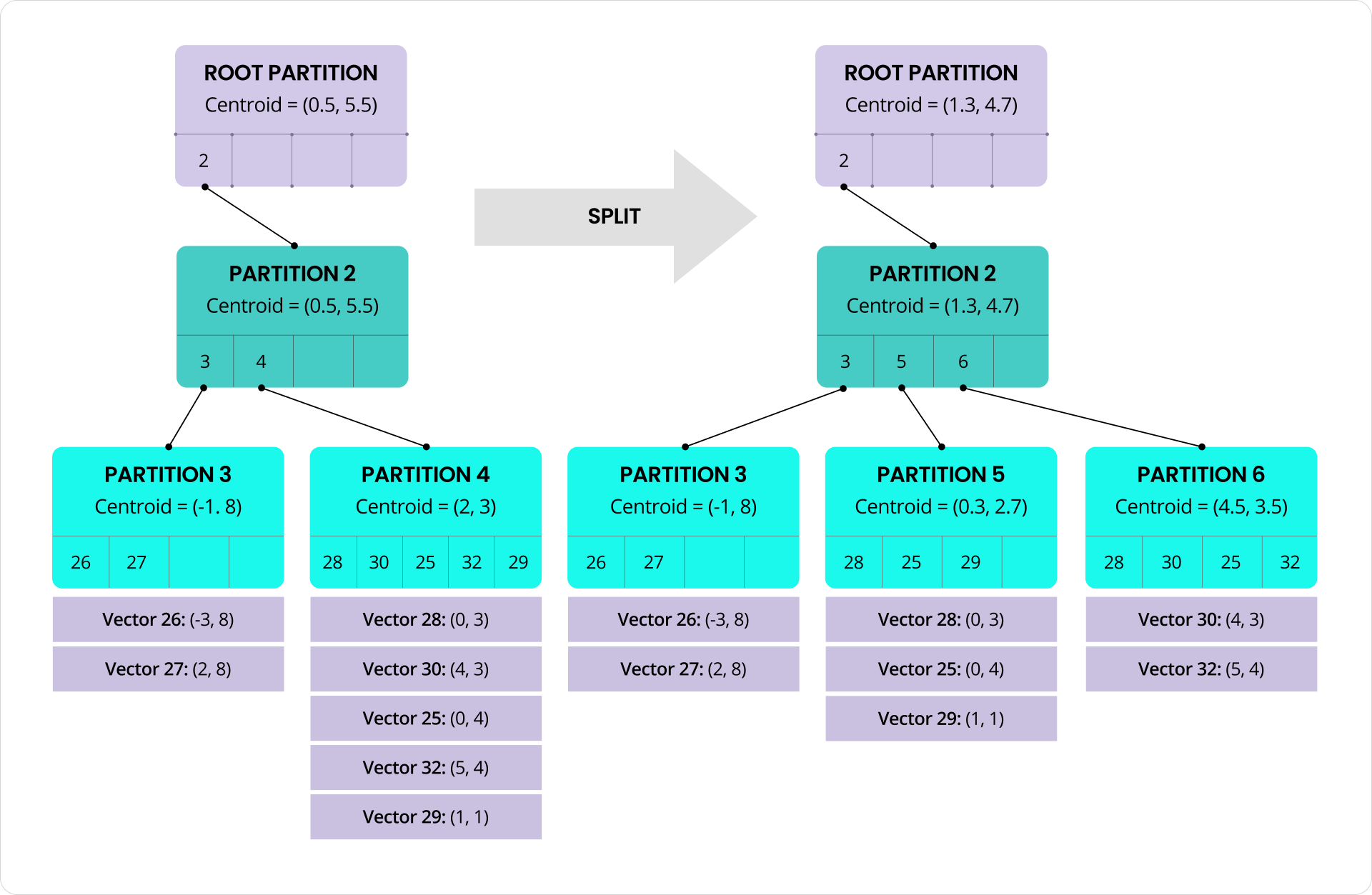
Splits happen automatically in the background to reduce impact on foreground transactions. When a split is triggered, the vectors in the original partition are divided into two roughly equal groups using a balanced variant of the K-means algorithm. Each group becomes a new, more tightly clustered partition with its own centroid. The tree is updated to reflect this change, and future inserts are routed to the new partitions based on proximity to these new centroids. Here’s an example where partition 4 is replaced by partitions 5 and 6 at the leaf level of the tree:
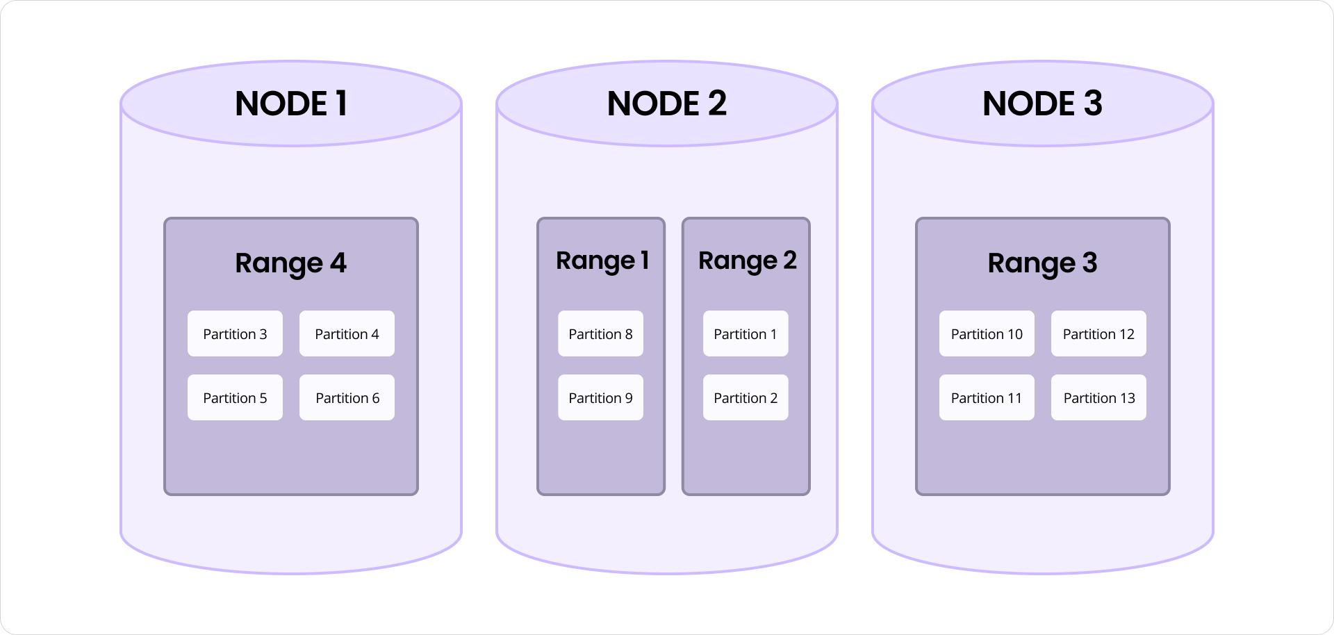
It’s also worth noting that partition splits are distinct from CockroachDB’s range splits, though the two work together to ensure scalability and consistent performance. A partition is a logical unit within the index that groups similar vectors. A range is a physical unit of storage in the key-value layer. Splitting a partition improves search efficiency by maintaining tight clustering of vectors. Splitting a range helps balance data storage and access across the cluster. Together, these mechanisms reduce hot spots and help spread both query and insert load more evenly. When nodes are added to the system, ranges containing index partitions are automatically distributed across the new nodes, allowing the total workload to scale out with the cluster at near-linear rates.
There’s one wrinkle worth noting: some vectors may no longer be in the “right” partition after a split. A vector in the splitting partition might be closer to a nearby partition’s centroid than to either of the new centroids. Likewise, a vector in a nearby partition might now be closer to one of the new centroids. In both cases, vectors need to be relocated to the partition with the closest centroid. To see how this can happen, consider these red and blue clusters (centroids are marked with X):
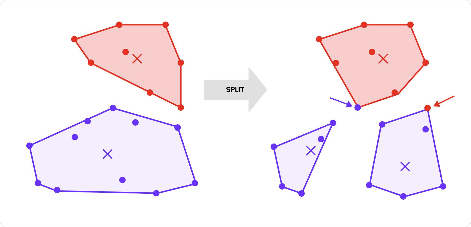
After the blue cluster is split, one of its vectors is reassigned to the red cluster because it’s now closer to the red centroid than to either of the new blue centroids. Similarly, one of the red vectors is reassigned to the righthand blue cluster for the same reason. Relocating vectors based on updated proximity is introduced in the SPFresh paper (as part of ensuring “nearest partition assignment”) and plays a key role in maintaining high clustering accuracy after splits.
While splits ensure that partitions don’t grow too large, merges ensure they don’t shrink too small. If vectors are deleted or moved such that a partition falls below the minimum size, a background process merges it away. Its vectors are reassigned to nearby partitions, and the original partition is removed from the tree.
Taken together, splits, merges, and partition reassignments are highly effective at preserving index accuracy, even after many cycles of vector inserts, updates, and deletes. In fact, the approach works so well that there's not a lot to gain from rebuilding the index after adding new data. You can start with an empty table, insert millions of vectors, and still get high accuracy. The index adapts rapidly and dynamically as the data evolves, keeping itself balanced and efficient over time.
Reducing Index Size by 94%
Full-precision vectors are expensive. OpenAI embeddings, for example, use 1,536 dimensions with 2-byte floats, which comes out to about 3 KB per vector. Multiply that by millions of vectors, and the index size adds up quickly. Storage is one cost, but often the greater expense is the CPU and memory required to load and scan full vectors during index searches.
To reduce this overhead, C-SPANN uses a technique called quantization to compress the vectors stored in the index. Instead of storing full vectors, it stores compact binary representations that approximate the originals. During search, distances are computed using these quantized forms, which are both smaller and faster to scan.
While many quantization algorithms exist, we use one called RaBitQ, which reduces each vector dimension to a single bit. It stores those bits along with a few precomputed values per vector, achieving roughly a 94% reduction in size for common cases. In the OpenAI embedding example, that shrinks a vector from about 3 KB to only around 200 bytes.
This approach integrates naturally with the K-means tree: each vector is quantized relative to the centroid of the partition it belongs to, allowing for tighter grouping and better accuracy. Because quantization is local to each partition, splits and merges only require re-quantizing the vectors within the affected partition. This enables the index to evolve incrementally and locally, without centralized coordination or global retraining.
While I won’t dive into every detail, I want to show you how beautiful and simple the core RaBitQ algorithm is. Each data vector is first “mixed” with a random orthogonal transform, which spreads any data skew more evenly across dimensions while still preserving angles and distances. It’s then mean-centered with respect to the partition centroid and normalized to unit length. Finally, each dimension is converted to a bit: zero if the value is less than zero, one otherwise.
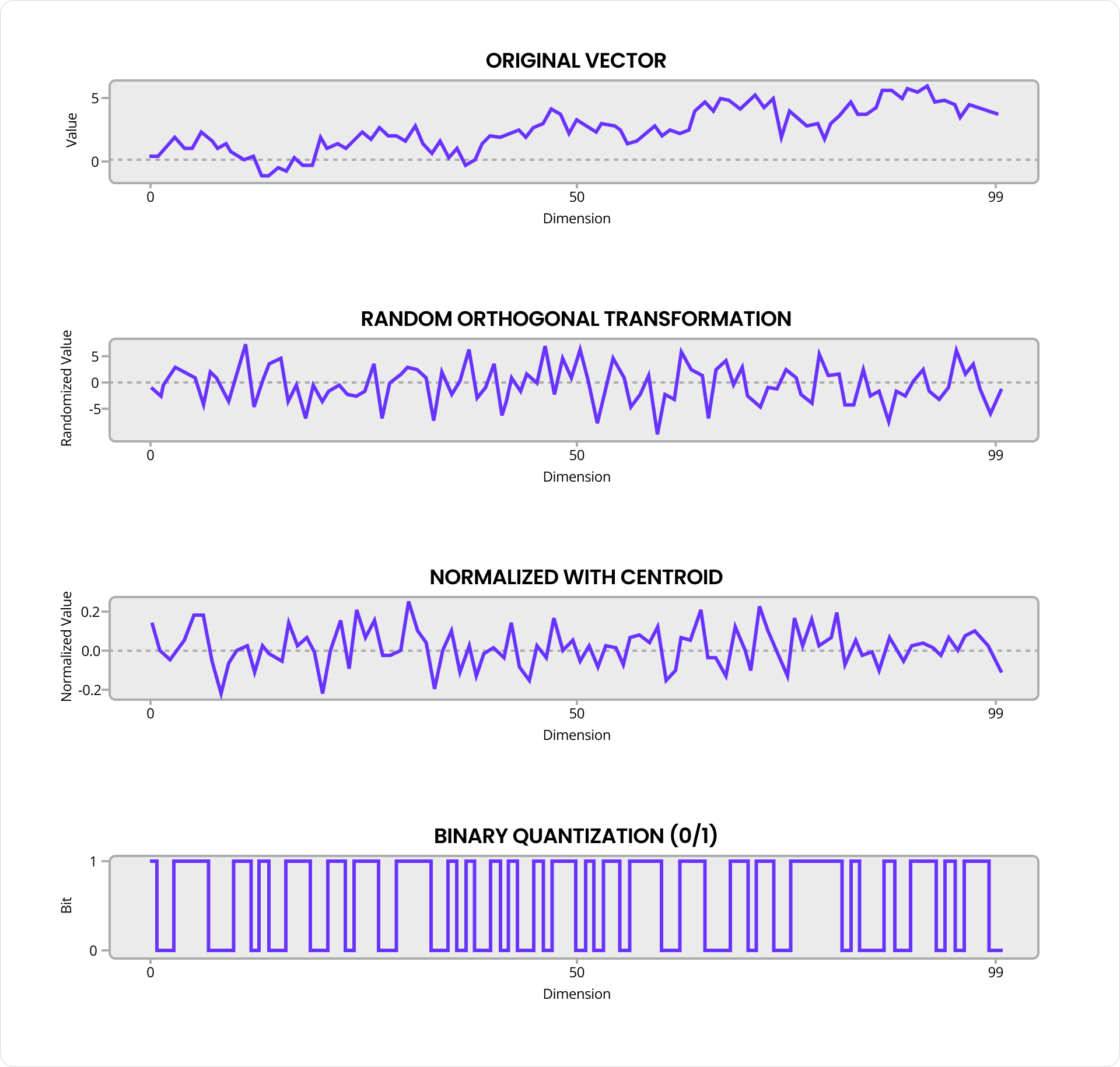
The result is a string of bits that captures the essence of the original vector in highly compressed form. These bits are stored alongside the dot product between the quantized and original vectors, as well as the exact distance of the original vector from the centroid. Remarkably, that’s enough to estimate distances with reasonable accuracy. To make distance comparisons fast as well as compact, RaBitQ uses a different quantization method for the query vector that assigns 4 bits per dimension and is optimized for SIMD instructions.
Since quantization is lossy, these distance estimates are only approximate. To correct for this, C-SPANN includes a reranking step. We scan quantized vectors to build a candidate set, then fetch the original full vectors from the table to re-compute exact distances. By over-fetching candidate vectors, we can compensate for quantization error. RaBitQ provides error bounds that help determine how many extra vectors are needed to find the true nearest neighbors with high probability.
The result is the best of both worlds: fast, compact scans with accurate results.
An Index for Every User
I’ve explained how C-SPANN can cluster vast numbers of vectors and keep the index fresh with real-time, incremental updates. But there’s a further twist to the story. In most real-world applications, those vectors belong to someone, whether it be a user, a customer, a tenant, or some other owner. And most queries are scoped to just that one owner. In fact, including vectors from other owners could be a security issue.
CockroachDB vector indexes handle this cleanly by supporting prefix columns, which allow the index to be partitioned by ownership (or anything else). Here’s a simple example:
CREATE TABLE photos (
  id UUID PRIMARY KEY,
  user_id UUID,
  embedding VECTOR(1536),
  VECTOR INDEX (user_id, embedding)
);
In this case, the vector index is partitioned by the leading user_id column. That means photo embeddings are indexed and searched per user. Here’s a query that finds the 10 closest photos for a given user, using pgvector compatible syntax:
SELECT id
FROM photos
WHERE user_id = $1
ORDER BY embedding <-> $2
LIMIT 10
Even if the index contains billions of photos, this query will only search the subset that belongs to one user. Performance for inserts and searches is proportional to the number of vectors owned by that user, not the total number of vectors in the system. Contention between users is minimized, since queries don’t touch the same index partitions or rows.
Behind the scenes, the index maintains a separate K-means tree for each distinct user. From the system’s perspective, there isn’t much difference between 1 billion vectors arranged in a single tree or the same number spread across a million smaller trees. Vectors are still assigned to partitions and packed into ranges in the CockroachDB key-value layer. Those ranges are automatically split, merged, and distributed across nodes, just like any other data, enabling near-linear scaling as usage grows.
Users in Every Region
Prefix columns become even more powerful when used with CockroachDB’s multi-region features. For example, you can use a REGIONAL BY ROW table to store each user's data in their home region, which reduces latency and helps meet data domiciling requirements:
CREATE TABLE photos (
  id UUID PRIMARY KEY,
  user_id UUID,
  embedding VECTOR(1536),
  VECTOR INDEX (crdb_region, user_id, embedding)
) LOCALITY REGIONAL BY ROW;
This statement automatically adds a crdb_region column to the table, which is included in the vector index alongside user_id and embedding. This ensures that both table and index rows are co-located in the region specified by each row’s crdb_region value. Photos for a user in Europe will be stored in Europe, with fast, local access from that region. Photos for a user in the US will be stored in the US, with equally low-latency access there. The combination of crdb_region and user_id as prefix columns partitions the index by both location and ownership, making it efficient, secure, and locality-aware by default.
Future Work
We released a preview of vector indexing in our 25.2 release. It includes all of the core functionality described above, but several optimizations are still underway to improve accuracy and performance. Merge operations and partition reassignments are not yet fully implemented. Root partition caching and expanded use of SIMD instructions will help speed up both searches and inserts. We're also working to minimize contention between foreground queries and background operations like splits and merges.
On the functionality side, we plan to expand support for IMPORT, ALTER INDEX and additional distance metrics. The current implementation supports Euclidean distance, and we’re actively working to add support for cosine and inner product as well. And while the current implementation can leverage the vector index when filtering on prefix columns, we’re aiming to support a wider range of WHERE clause filter patterns in future releases.
If you're working with a large number of vectors, need to support high QPS, fresh results, geo-locality, high-availability, or anything else discussed here, we'd love to hear from you. Your use case could help shape our future roadmap.