A Reference Architecture for a Next Generation Global Reporting Platform

In Part 1 of this article series on Global Reporting Platforms, we explored why traditional reporting architectures are increasingly unable to keep up with modern business demands. Systems built around batch pipelines, replicated copies, and loosely coordinated components struggle as reporting becomes more operational, more distributed, and more tightly governed. The symptoms are familiar: lagging data, inconsistent metrics, brittle pipelines, and growing operational overhead.

In Part 2 we move from concept to practice. Rather than revisiting why reporting platforms must evolve (refer back to Part 1), now let’s focus on how they can be designed differently. Follow along for a concrete reference architecture built on CockroachDB that shows how reporting, historical access, and semantic query patterns can be supported directly on operational data. There’s no need to stitch together separate systems to make the platform behave coherently.

This article is intentionally practical. I’m not benchmarking performance, comparing vendors, or cataloging features. This working architecture walkthrough demonstrates how transactional ingest, data archiving, reporting queries, point-in-time views, and vector-powered access patterns can coexist in a single operational database. You’ll get valuable tips on: 

• configuration 

• data placement 

• workload isolation 

• observable behavior

How can you make the most of this global reporting platform setup guide?

The accompanying GitHub repository and demo environment make these ideas tangible. They show how different workloads can be isolated using regions, hardware profiles, and access paths; how reporting can be decoupled from transactional traffic without duplicating data; and how historical and semantic queries can run directly against consistent operational state. Together, they provide a practical starting point for teams looking to rethink how reporting platforms are built. You’ll gain clarity on what should reasonably be expected from an operational system of record.

Think of this as a reference architecture, rather than a prescriptive template. While specific region layout, sizing choices, and lifecycle boundaries are intentionally precise, so their effects can be observed and reasoned about, in a real system, those choices would be driven by regulatory, operational, and cost constraints.

Don’t think of this specific setup as something to copy verbatim. The goal here is to make workload intent, placement policy, and tradeoffs visible. Prioritize your understanding of why each boundary exists, rather than the exact enforcement mechanics .

Lastly, readers familiar with distributed databases and reporting architectures will recognize many of the individual components; the value here lies in how they are composed and where responsibility is placed.

Architecture Overview

This reference architecture is a single CockroachDB cluster deliberately shaped to support different reporting-related workloads without splitting data across systems.

Note, that the cluster is not uniform. Nodes are grouped into regions with explicit roles, different hardware profiles, and different access paths. The goal is to keep data in one place, while ensuring that transactional ingestion, archival storage, and reporting queries do not interfere with each other.

At a high level, the cluster consists of:

• Three transactional regions (tx1, tx2, tx3)

• Three archive regions (ar1, ar2, ar3)

• One reporting region (report)

All CockroachDB regions participate in the same cluster and share the same schema:

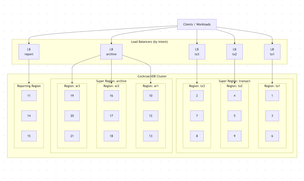
_{A reference architecture illustrating how transactional ingest, historical retention, and reporting queries can be isolated by region and access path within a single CockroachDB cluster, reducing architectural sprawl.}

In CockroachDB, a region is a logical grouping of nodes. Although regions often align with cloud provider regions in a given deployment, they are a database-level abstraction and can also be used to group nodes by purpose or role.

A Super Region is a CockroachDB abstraction that groups three or more regions together for the purpose of domiciling data.

In our architecture depicted above, there are the following regions and super regions:

Related

Learn how to design resilient, multi-region data architectures where operational workloads, reporting, and history all run on the same system of record.

The blueprint to deliver distributed data at scale

Regions as policy, not geography

Regions in this architecture are used primarily as policy boundaries, not just geographic ones.

Transactional regions, archive regions, and the reporting region exist because they serve different purposes, run on different hardware, and have different expectations. Super regions are used to group regions with similar lifecycle and cost characteristics, allowing data to move between them without changing schemas or application logic.

This approach replaces traditional reporting pipelines with placement and replication decisions inside the database. Data does not become “reporting data” because it was copied somewhere else. It becomes reporting data because it is queried through a different access path and executed on different resources.

To see how these multi-region and data-locality patterns show up in a real deployment, this talk walks through CockroachDB powering a multi-region, compliance-sensitive application:

Transactional regions

The transactional regions handle application ingest.

Each transactional region consists of multiple modestly-sized nodes. These nodes are sized to handle concurrent writes and steady update rates rather than large scans or heavy aggregation.

Data written by the application is placed using regional-by-row locality, so inserts land close to where they originate. Transactional regions are grouped into a transactional super region, which defines replication and placement policy for hot data.

In our reference architecture, there are three transactional CockroachDB regions. These regions are aligned with three different geos (usually three cloud regions, e.g. in the case of AWS could be us-east-2, eu-central-1, us-west-1). The nodes in each of these CRDB regions are fronted with a separate load balancer. Applications running in the specific geo will prefer to connect to the CRDB cluster via the load balancer that is geographically the closest.

Archive regions

Archive regions exist to hold historical data with different cost and performance characteristics.

Nodes in archive regions are smaller and denser. They are not optimized for write throughput or low-latency reads. Instead, they are sized to retain large volumes of data economically while remaining queryable.

Data is moved into archive regions explicitly as part of its lifecycle. Archiving is done by domiciling data into an archival super region, not by exporting and re-ingesting it elsewhere. Once archived, the data remains part of the same database, with the same schema and semantics.

Archive regions are accessed through their own entry point, so long-running historical queries do not interfere with transactional ingest.

Reporting region

The reporting region is built differently from the rest of the cluster.

It consists of a small number of very large nodes, sized primarily for CPU and memory. These nodes are intended to absorb read-heavy workloads: dashboards, historical queries, point-in-time views, and exploratory access.

The reporting region does not exist to store primary copies of transactional data. Instead, it exists to execute queries efficiently against data that lives elsewhere in the cluster. Reporting queries enter the system through a dedicated reporting endpoint that routes traffic toward these nodes.

This separation allows reporting workloads to scale independently. Increasing reporting capacity does not require scaling transactional regions, and vice versa.

Explicit access paths

A key characteristic of this architecture is that workload intent is explicit at connection time.

Transactional traffic, reporting queries, and archival access each use separate endpoints. This avoids relying on query classification or runtime heuristics to guess intent after the fact. If a dashboard connects to the reporting endpoint, it will not compete with application writes simply because someone misconfigured a connection string.

This makes capacity planning, troubleshooting, and failure analysis much simpler. Each class of workload is visible, isolated, and independently tunable.

Schema and Data Model (Transactional Focus)

Let’s start the walkthrough with the database and schema, because everything that follows – placement, locality, lifecycle – is a direct consequence of how the data model is defined.

At this stage, we’re focusing exclusively on transactional ingest. Archival behavior and reporting surfaces come later.

Database overview

All examples in this walkthrough use a single database called nextgenreporting.

The database is intentionally small. The goal here isn’t to model a full production schema, but to make transactional behavior easy to reason about and observe as load is applied.

Core tables and why they exist

The schema consists of three tables:

• geos

• stations

• datapoints

Each one exists for a specific reason. Visit this github for more details.

geos

The geos table models conceptual geography and its association with transactional regions.

In a real deployment, this mapping would be implicit. Physical devices connect through region-specific load balancers, and the gateway node determines placement automatically. In this walkthrough, we’ll model that specific mapping so we can drive and explain placement deterministically.

Each geo maps to a transactional region (tx1, tx2, or tx3). The table is small, static, and marked GLOBAL.

A GLOBAL table in CockroachDB is replicated across all regions and optimized for low-latency, strongly consistent reads from any location (visit our global table docs page here). Because this table contains read-mostly reference data with infrequent updates, the additional coordination cost on writes is minimal while every region benefits from fast local access.

stations

The stations table represents physical data sources.

Each station belongs to a geo and acts as a stable identifier that produces datapoints over time. We’ll use stations to introduce realistic cardinality and fan-out: many independent sources, each generating a stream of data.

Like geos, this table is also marked GLOBAL. Stations are referenced during ingest, but they are not write-heavy themselves.

The datapoints table

The datapoints table is where most of the action happens:

Each row represents a single datapoint produced by a station at a specific point in time. Structurally, it behaves like a high-ingest, time-oriented fact table.

A few design choices are worth calling out:

• The primary key is at, station which models a natural time-series pattern per station and provides a stable sharding key.

• Scalar columns param0 through param4 represent typical numeric or categorical measurements.

• param5 is a JSONB column used to model semi-structured attributes that evolve over time.

• param6 is a vector column, included for later steps, but not yet relevant to transactional behavior.

Notice now the primary key uses USING HASH with a defined bucket count 16 to prevent write hotspots. In time-series patterns, monotonically increasing timestamps can concentrate inserts into a small number of ranges, creating contention and uneven load distribution. Hash-sharding distributes writes across multiple buckets, spreading ingest evenly across nodes and maintaining stable throughput under high concurrency.

Regional-by-row locality

The datapoints table is defined as REGIONAL BY ROW (more info here), using a hidden crdb_region column as the locality key.

This means each row is explicitly placed into a transactional region (tx1, tx2, or tx3), and stored and replicated according to that region’s policy.

In a production system, this column would typically default to gateway_region(), letting network topology determine placement implicitly. In this walkthrough, I populate it explicitly so placement behavior is deterministic and easy to verify.

At this point in the walkthrough, all rows land in transactional regions only. Archival and reporting regions aren’t involved yet.

Transactional super region (context)

All transactional regions are grouped into a transactional super region, which defines replication and survivability for hot data.

We don’t go into lifecycle transitions here – the core point is simply that transactional data shares a common placement and replication policy.

Transactional workload generations

To drive ingestion, let’s use a custom dbworkload (available here) class called `Datapointtransactions`.

This class exists to emulate what would normally be done by real devices connecting through region-specific load balancers.

Each executing thread repeatedly:

1. Selects a station

2. Generates a synthetic datapoint

3. Upserts that datapoint into the datapoints table

By default, this workload class will evenly distribute newly generated rows in the `datapoints` table among the three transactional regions tx1, tx2 and tx3. Since we don’t rely on the physical location placement of the transactional regions and their associated load balancers, but still may want to drive the region targeted workloads and observe the data placement behavior.

This workload class accepts an optional region argument:

• args = { "region": "tx1" }

When we pass this argument, the workload restricts station selection to geos mapped to that transactional region. The crdb_region column is set accordingly, and all generated datapoints land in the specified region.

What to observe at this stage

After completing this step, we can observe:

• Continuous transactional ingest into the datapoints table

• Rows landing in the expected transactional regions

• A clear, inspectable relationship between station, geo, and row placement

So far the system consists purely of transactional data in transactional regions. Everything that follows in the walkthrough builds on this foundation.

After running some transactional workloads, we can now observe the domiciling of the rows in the datapoints table: 

 The output should look like this:

There is also a convenient utility show_ranges.py in the CockroachDB reporting GitHub repository.

The sample output below clearly shows:

• how many rows each range contains

• which region holds the leaseholder

• where replicas are placed

Now get ready for…

How can data be archived without pipelines or data movement?

Once transactional ingest is in place, the next concern is data lifecycle.

In this model, datapoints are written into transactional regions (tx1, tx2, tx3) and are assumed to be mutable for a short time . After that grace period, the rows are considered stable: They are no longer updated, but they must remain queryable. The goal shifts from write locality and low latency to cost-effective retention with clear survivability guarantees.

In this walkthrough, let’s treat that grace period as one month. Anything older than that is eligible for archiving.

Archival regions and survivability assumptions

Archival data lives in a separate archive super region, made up of three archive regions: ar1, ar2, and ar3.

There are two reasons for this structure:

1. We want to use a super region to enforce domiciling rules for archived data. In CockroachDB, a super region requires at least three regions.

2. We define the survival goal as regional survival, which means each archive region must be able to tolerate node-level failures independently. In practice, that means each archive region is backed by at least three nodes.

What’s important is not the exact sizing, but that archival data follows a different placement and survivability policy than transactional data, while still living in the same table.

Related

Explore how leading organizations are re-architecting for always-on operations -- and what outages really cost when reporting is on the critical path:

The State of Resilience 2025

Archiving as a placement change

Archiving in this architecture is not implemented as an export, a copy, or a pipeline. Instead, it is a placement change.

Rows are archived by changing their crdb_region value from a transactional region (tx1, tx2, tx3) to an archive region (ar1, ar2, ar3). That single change is enough to trigger CockroachDB to re-replicate and re-domicile the affected ranges according to the archive super region’s policy.

Neither the schema or the table changes. The data remains queryable throughout the process.

The archive_datapoints() stored procedure

We implement archiving as a SQL-callable stored procedure called archive_datapoints().

The procedure works in small batches and loops until no more eligible rows remain. Each iteration:

• Selects up to 1,000 datapoints that:

  • currently live in transactional regions

  • are older than one month

• Chooses an archive region

• Updates only the crdb_region column for those rows

Because this runs as standard SQL, I can invoke it directly from the SQL shell:

The procedure is incremental, online, and idempotent. There is no downtime window and no coordination with application traffic:

It is important to understand the internal mechanics of changing the value of the crdb_region column (type public.crdb_internal_region) in the REGIONAL BY ROW table. The current value in such a column drives the physical placement of the data range containing the row’s data. When crdb_region changes from tx1 to ar2, CockroachDB will relocate the row’s data to a data range domiciled in the ar2 region.

Archive region selection (demo behavior)

This stored procedure distributes archived rows randomly across ar1, ar2, and ar3. This is intentional, but it’s important to be precise about why we take this approach:

The goal here is not to model a production data-placement policy. Instead, we want to demonstrate super-region placement and survivability behavior so it’s easy to observe. Random distribution ensures that archived ranges spread across all archive regions, making the resulting placement immediately visible.

In a real-world system, archive region selection would typically follow explicit business, compliance, or cost rules.

Verifying archival placement

To verify that archiving is doing what we expect by running `show_ranges.py` as described earlier.

After running the archive procedure, the output clearly shows two populations coexisting in the same table:

• Ranges whose leaseholders and replicas live in tx* regions

• Ranges whose leaseholders and replicas live in ar* regions

At this point, nothing has been copied, no secondary table exists, and no reporting store has been populated. The only thing that has changed is where the archived  rows are located  and which resources serve them.

What this step demonstrates

After this step, the system has:

• Active transactional data in transactional regions

• Stable historical data in archive regions

• A single table spanning both

• No pipelines, exports, or re-ingest jobs

Most importantly, this transition happens inside the database, using standard SQL, and remains fully observable. Everything that follows – reporting behavior, historical queries, and isolation – builds directly on this placement change.

Now we’re really gaining momentum! It’s time to start…

How can reporting work without replicas or ETL pipelines?

Context: Mixed Workloads on Legacy Databases

In many legacy database architectures, reporting runs directly on the same systems that ingest transactions. As reporting demands grow, the typical response is to introduce workload managers: priority classes, throttling rules, concurrency limits, or time-of-day policies intended to keep analytical queries from overwhelming transactional workloads. 

These mechanisms can mitigate contention, but they do not remove it. All workloads still compete within the same execution domain, buffer pools, and coordination paths.Then, as data volumes grow, arbitration increasingly turns into stalled queries, timeouts, or failed jobs. 

The approach described in this global reporting platform setup walkthrough takes a different stance. Rather than forcing one system to behave like two through scheduling and throttling, it separates work by intent at the architectural level – allowing transactional ingest and reporting queries to execute on different resources while remaining anchored to a single, consistent source of truth.

With transactional ingest and archiving in place, the next step is reporting.

In this architecture, reporting is handled by a dedicated reporting region called “report.” This region is intentionally shaped differently from the rest of the cluster, both in terms of hardware and how it’s used.

The reporting region

The reporting region consists of three nodes, each significantly larger than the nodes in transactional and archive regions.

Two constraints are intentional and important:

• No rows from the datapoints table are domiciled in the reporting region

• The reporting region exists purely to execute read-only queries

The reporting region does not store primary data, nor does it host replicas for transactional or archival ranges. Its role is not data locality, but compute isolation: providing CPU and memory for complex queries without competing with ingest or lifecycle operations.

Why do reporting queries require a different execution model?

The queries we run from the reporting region are fundamentally different from transactional operations.

They typically involve:

• Multi-table joins

• Common table expressions (CTEs)

• Aggregations and grouping

• Ordering across large result sets

• Time-based rollups over large windows

These queries take longer to execute than typical INSERT, UPDATE, or DELETE operations. More importantly, they do not need to reflect the latest millisecond of data. What they do require is a consistent, repeatable view of the data across all tables involved in the query.

That makes them a good fit for CockroachDB’s multi-version concurrency control (MVCC) model and the AS OF SYSTEM TIME feature.

Stable snapshots with AS OF SYSTEM TIME

All reporting queries in this walkthrough are executed using:

This has two effects.

First, the query executes at a fixed MVCC timestamp, so it observes a consistent snapshot of the database, regardless of concurrent writes or archival activity.

Second, because the query is historical, it does not require coordination with the leaseholder. The database is free to serve reads from any up-to-date replica for each range involved in the query.

It’s important to be precise on this point: the replicas being read are not located in the reporting region. They live in the transactional and archive regions where the data is domiciled. The reporting region provides the gateway where the bulk of query execution occurs, while the data itself is read from follower replicas elsewhere in the cluster. Some operations (such as filtering and certain aggregations) are pushed down to those replicas, but the majority of the query’s coordination, ordering, and merge processing is performed by the gateway.

This separation is intentional, because it decouples query execution from data placement.

Reporting workload generation

To generate reporting load, let’s use a separate dbworkload class called Datapointreporting.

This workload is executed only against the load balancer fronting the reporting region. Reporting queries never connect to transactional or archive endpoints.

Each executing thread cycles through a fixed set of read-only queries that exercise common reporting patterns. The workload does not mutate data and does not rely on any region-specific assumptions beyond read access.

Example reporting queries

The workload includes queries such as:

• Counting stations by transactional region

• Aggregating datapoints by region

• Rolling up datapoints by hour for the current day

• Rolling up datapoints by day over the last year

Each query:

• Joins across datapoints, stations, and geos

• Uses AS OF SYSTEM TIME follower_read_timestamp()

• Executes on compute in the reporting region

• Reads data from follower replicas in transactional and archive regions

These queries are deliberately representative, rather than optimized. The goal is to demonstrate behavior under realistic reporting patterns, not to micro-benchmark execution speed.

What to observe at this stage

When running the reporting workload, we observe:

• Reporting queries consuming CPU and memory in the reporting region

• No impact on transactional ingest latency

• No coordination with transactional leaseholders

• Stable, repeatable results across runs

• Clear separation between where data lives and where queries execute

At this point, the system supports three distinct behaviors on the same dataset:

• Transactional writes in transactional regions

• Lifecycle transitions into archive regions

• Read-only reporting queries executed in a dedicated reporting region

No data has been copied. No reporting replica has been created. The separation is achieved entirely through access paths, placement policy, and MVCC-based snapshots.

Materialized Views in the Reporting Region

At this point in the walkthrough, reporting queries are already isolated from transactional ingest and archival activity. The next step is not about freshness or consistency, since those are already handled by MVCC and historical reads.

There’s a problem at this stage that materialized views solve: shape.

Materialized views let us pre-shape data for reporting, without changing the transactional or archival model.

They allow us to:

• collapse joins that are semantically stable

• index derived attributes that would never make sense on transactional tables

• apply reporting-specific placement and lifecycle rules

• while remaining transactionally and semantically coupled to the source of truth, rather than detached through pipelines or duplicated stores.

This distinction matters: The materialized view is not a reporting copy produced by ETL. Instead, it’s a derived structure that stays consistent with the underlying data and evolves with it, under the same transactional guarantees.

Creating the reporting materialized view

Let’s start by defining a materialized view that joins the core transactional tables into a reporting-friendly projection:

This view does not introduce new semantics. It fixes a shape that reporting queries were already asking for repeatedly: resolved joins, explicit columns, and a stable projection that includes both scalar attributes and vectors.

Out of the box, however, the view is only logically correct.

Aligning the view with the reporting region

By default, a materialized view inherits generic placement rules. That means its ranges can be distributed across transactional and archive regions, which is not what we want for a reporting artifact.

So the next step is to make the intent explicit and contain the view entirely within the reporting region:

A few choices here are deliberate:

• All voters and replicas live in the report

 The materialized view becomes self-contained. Both query execution and data access stay within the reporting region.

• Region failure makes the view unavailable

 That’s acceptable. This view is not a source of truth.

• Short GC TTL

We can also verify the associated data range domiciling using show_ranges.py:

We don't need long point-in-time recovery for a derived structure. A shorter TTL reflects the fact that the view can always be rebuilt, and keeping storage churn under control.

At this point, the reporting region owns its reporting data explicitly, without affecting the placement of transactional or archival data.

Refreshing the view

Materialized views don’t update automatically. Refreshing is explicit:

This is intentional. Refreshing acts as a control point, which lets us decide when reporting data advances and how often expensive recomputation happens. In practice, this means we can align refresh cadence with reporting needs rather than with ingest velocity.

Indexing for reporting, not ingest

Once the view is in place, we can treat it like a reporting table. We can add indexes that would be inappropriate on a high-ingest transactional table, without worrying about write amplification or contention. For example, we can create functional indexes:

These indexes exist purely to serve reporting queries –  they don’t affect transactional ingest or archival transitions.

We also create a vector index on the materialized view:

This gives us a semantic access path that is separate from live operational vector queries.

Live vs materialized vector search

With the materialized view in place, the system supports two distinct vector query modes.

Live vector search answers:

 “What does the system look like now?”

These queries run directly against the base datapoints table, using historical snapshots to avoid interfering with writes.

Materialized view vector search answers:

 “What did the system look like then, in a curated form?”

While it’s possible to issue multiple AS OF SYSTEM TIME queries directly against the base table, each such query must still resolve joins, scan large datasets, and operate under transactional indexing constraints.

Materialized views let us :

• precompute the reporting shape once

• index it specifically for semantic access

• compare curated snapshots efficiently over time

The value here is not raw performance. As we’ll see in this demo environment, the difference is modest. The value is semantic clarity, repeatability, and isolation.

Related

See how distributed SQL and vector search let us run semantic search and AI workloads directly on operational and historical data. 

The New Blueprint for AI-Ready Data Vector Search Meets Distributed SQL

Storage and cost considerations

Materialized views can consume significant storage, especially if multiple views or refresh points are maintained.

In this global reporting platform architecture, that cost is intentional and contained:

• All materialized view data lives in the reporting region.

• Reporting nodes are sized for CPU and memory and can use storage optimized for read-heavy workloads.

• Range sizing and compaction strategies can be revisited independently from transactional tables.

This is a deliberate tradeoff: a controlled amount of storage in one place in exchange for avoiding separate reporting databases, ETL pipelines, and duplicated semantic layers.

In a production system, we would also revisit range sizing for reporting views, since their access patterns differ significantly from transactional tables. That tuning is orthogonal to the core architecture and can be validated independently.

What this step demonstrates

With materialized views in place, the reporting architecture now has:

• A transactional source of truth

• Archived historical data

• A reporting-only, pre-shaped semantic surface

• Independent indexing and lifecycle rules

• Explicit control over refresh and snapshot boundaries

This all happens inside the same database, without breaking transactional consistency or introducing detached copies of the data.

That is the real role of materialized views here: not speed, but architectural separation of concerns with preserved truth.

How can semi-structured data be queried without breaking the data model?

Structured data rarely stays fully structured.

In real systems, new attributes show up long before anyone knows what they mean or how they should be modeled. They’re often irregular, noisy, or only relevant to a subset of use cases. They’re not critical to day-to-day application behavior, but they are valuable – especially once patterns begin to emerge.

This is where many data architectures go off the rails.

The moment that semi-structured data appears, the default reaction is to introduce a second system: a document store, a search engine, or a lake. That decision is usually framed as “flexibility,” but in practice it fragments the data model. By the time the organization understands which attributes matter and how they should be structured, the data is already detached from the source of truth, delayed by pipelines, or transformed beyond recognition.

In this architecture, we take a more conservative approach. Instead, we keep semi-structured data attached to the SQL source of truth, even while its shape is still in flux. JSONB gives us a place to store attributes we don’t fully understand yet, without forcing premature schema decisions. More importantly, it lets us explore and analyze that data in context, alongside the structured fields that already drive the system.

The reporting materialized view is the right place to do this.

Because the view is isolated from transactional ingest, we can safely index and query JSONB without impacting write performance or lifecycle transitions. For example, we can inspect the raw shape of incoming attributes:

We can ask simple shape questions, such as whether a given key exists:

Or reason about nested structure:

To support these queries efficiently, let’s add an inverted index on the JSONB column:

The important point isn’t that JSONB exists – it’s where and how it’s used.

This data remains transactionally and semantically coupled to the rest of the system – not exported, flattened, or duplicated. When certain attributes stabilize and become operationally important, we can promote them into structured columns without reconciling multiple systems or re-deriving history.

Vectors follow the same pattern.

Both JSONB and vectors are outliers in the SQL world, but they solve the same problem: representing information that’s difficult to model upfront, yet critical to understand later. By keeping them inside the database – and on a reporting-only surface – we absorb uncertainty, explore meaning, and evolve the schema deliberately. All this, without paying the coordination cost of a second system.

This kind of architectural conservatism is often what saves teams from chaos and long-term cost.

Historical Extracts and Controlled Egress

In addition to interactive reporting, many systems need to perform large historical extracts. These are not dashboards and they’re not latency-sensitive queries. They are bulk reads used for downstream processing, analytics, model training, or regulatory purposes.

In this architecture, historical extracts are treated as first-class read workloads, not a special case that requires a separate data pipeline.

Extracts as snapshot reads

All historical extracts in this walkthrough are executed using:

This guarantees that each extract runs against a stable snapshot of the database. The snapshot is consistent across all joined tables, even if ingest and archiving are happening concurrently. That property is essential for bulk exports: The extract should reflect a coherent view of the data, not a moving target.

Full and filtered historical extracts

To model these workloads, we’ll use a separate dbworkload class called Datapointhistoricextract.

The workload executes two representative extract patterns.

The first is a full extract, reading all datapoints:

The second is a filtered historical extract, restricted to archived data:

Both queries join the same core tables and return large result sets. The difference is purely in scope.

Batched consumption

Rather than loading the full result set into memory, the workload consumes results in batches using Polars:

This models how real extract jobs behave in practice:

• streaming results

• bounded memory usage

• predictable resource consumption

The database is responsible for serving the snapshot, while the client controls how aggressively it consumes that snapshot”.

Where extracts run

One important aspect of this architecture is that extracts are not tied to a single execution location.

The same workload can be run:

• from the reporting region, when extracts involve complex joins or benefit from high CPU and memory, or

• from archive regions, when the extract is dominated by scanning archived data and proximity matters more than compute.

In both cases:

• the snapshot semantics are the same,

• no data is copied,

• and transactional ingest remains isolated.

The choice of execution location becomes an operational decision, not an architectural constraint.

What this step demonstrates

After this step, the system supports:

• Large, consistent historical reads

• Full or filtered extracts without pipelines

• Batched, memory-safe consumption

• Flexible execution placement

• No impact on transactional ingest

Most importantly, extracts operate directly on the same data and same semantics as reporting and operational queries. There is no “export schema,” no transformation step, and no secondary copy to reconcile.

This keeps downstream systems aligned with the source of truth while avoiding the operational overhead of maintaining separate extraction pipelines.

Changefeeds (CDC) as an Explicit Boundary

Change Data Capture is core to the CockroachDB story. It’s how data leaves the database when it truly needs to participate in external systems: stream processors, search indexes, audit pipelines, or downstream analytics platforms.

At the same time, CDC isn’t free: It introduces real work inside the database, and that work has architectural consequences. In this walkthrough, the goal is not to hide those costs, but to place them deliberately.

Enabling CDC

Before creating a changefeed, rangefeeds must be enabled:

We then create a changefeed on the datapoints table, emitting resolved timestamps and pinning execution to the reporting region:

A few choices here are intentional:

• CDC is enabled explicitly – it is not a background default.

• Resolved timestamps are enabled, so downstream consumers can reason about completeness.

• Execution is pinned to the reporting region, not to transactional regions.

What CDC actually observes

Once the changefeed is running, it emits two kinds of messages:

• Resolved timestamp messages, indicating progress of the feed

• Row change events, reflecting inserts and updates

When I insert a new datapoint via the transactional workload, the changefeed emits an after image of the row. When I run the archiving procedure and rows move from transactional regions into archive regions, the changefeed emits UPDATE events reflecting that lifecycle transition.

This is an important point: CDC does not just observe ingestion. It observes data lifecycle, including placement changes. Downstream systems can see when data moves from hot to archival storage and react accordingly.

Observed behavior under load

With CDC enabled and resolved timestamps turned on, we may observe serializable transaction retries during bulk archival operations:

• ReadWithinUncertaintyIntervalError

• RETRY_SERIALIZABLE

These errors did not appear before CDC was enabled.

This is expected behavior in a strictly serializable, MVCC-based system. CDC does not write data, but it tightens the timestamp invariants the database must uphold. With resolved timestamps enabled, the system must conservatively prove that no writes can appear before a given point in time. Under bulk updates, that additional coordination can surface as transaction retries.

Importantly, these retries are not failures. They are the mechanism CockroachDB uses to preserve correctness.

Why execution locality still matters

Pinning the changefeed to the reporting region does not eliminate CDC’s impact on transactional data. Writes still happen in transactional regions, and correctness constraints still apply cluster-wide. What execution locality does control is where CDC coordination and overhead run.

In this setup, we verify that the changefeed job coordinator runs on a node in the reporting region. That means:

• job scheduling

• resolved timestamp advancement

• retry loops

• buffering and encoding

• Kafka sink I/O

are all executed on infrastructure sized and intended for non-transactional workloads.

The cost of CDC still exists, but it’s absorbed intentionally, rather than competing directly with transactional ingest.

What this demonstrates

This setup demonstrates a few key architectural points:

• CDC is powerful and first-class, but not free.

• Enabling resolved strengthens guarantees and can surface serialization retries under bulk updates.

• CockroachDB preserves correctness by retrying, not blocking or weakening isolation.

• Execution locality does not remove CDC’s constraints, but it controls where the complexity lives.

CDC is not how reporting works in this architecture, and it is not required for lifecycle management. It is the explicit boundary where data leaves the database, and where the cost of doing so is paid knowingly. That distinction is what keeps the rest of the system simple.

Reporting as an Operational Property, Not a Pipeline

The global reporting platform architecture in this article is not a new reporting product, and it is not a shortcut around hard problems. It is a different way of deciding where those problems belong.

Traditional reporting stacks push complexity outward: They externalize lifecycle management into pipelines, consistency into replication logic, historical access into secondary stores, and performance into caches. Each step appears reasonable in isolation. Collectively, however, they turn reporting into a coordination problem that tangles teams, systems, and time.

This distributed SQL reference architecture, demonstrated using CockroachDB, takes the opposite approach. It pulls reporting concerns inward – into the operational database itself – and treats them as first-class properties rather than downstream obligations.

In this paradigm transactional ingest, historical retention, reporting queries, point-in-time views, and semantic access all operate on the same data, under the same consistency model, with explicit isolation and observable tradeoffs. Data does not become “reporting data” because it was copied or transformed: It becomes reporting data because it is accessed differently, executed on different resources, and governed by different placement and lifecycle policies – all within a single system.

That shift has practical consequences:

• Reporting does not depend on pipelines to be correct.

• Historical queries do not require shadow schemas.

• Performance isolation is achieved through topology and access paths, not guesswork.

• Changefeeds become an explicit boundary, not a hidden dependency.

• Schema evolution and data lifecycle remain operational concerns, not reporting outages.

None of this removes the need for careful capacity planning, indexing, or workload tuning. What it removes is the need to rebuild correctness at every layer of the stack.

For teams designing next-generation reporting platforms – especially in environments where correctness, auditability, and global access are non-negotiable – the most important question is no longer “How do we move the data?” It is “Why does reporting require a different system at all?”

CockroachDB does not eliminate reporting complexity. It relocates it, into a system designed to handle it continuously, transactionally, and transparently. The result is not just fewer components, but a platform where reporting behaves like an operational capability rather than an afterthought. 

What begins as a reference architecture for a next-generation global reporting platform reveals something broader once it is implemented in practice: Supporting SQL queries, historical access, semi-structured data, and semantic search directly on operational data forces reporting concerns – consistency, isolation, lifecycle, and cost – to be addressed at the architectural level, rather than pushed into downstream systems. 

When it works through those constraints, reporting stops being a separate stack and instead becomes an operational property of the system itself. The impact on enterprises is powerful: They don’t just gain a more capable reporting platform, but an advanced architecture that allows reporting, history, and evolving data requirements to coexist – without fragmenting data or multiplying systems as complexity grows.

Ready to learn more about making CockroachDB your global reporting platform? Visit here to speak with an expert.

Alex Seriy is a Senior Staff Sales Engineer at Cockroach Labs, where he designs and builds reference architectures that explore how distributed systems behave under real operational constraints. His work centers on questions of correctness, data lifecycle, workload isolation, and governance in globally distributed SQL systems. By grounding theory in observable system behavior, he helps teams reason about architectural responsibility rather than assembling downstream compensations.